How to Calculate Due Dates with Google Sheets
Say the date today is the 12th of August 2022. If I were to ask you what the date is tomorrow and the date the day after, you’d be able to figure it out quickly without much calculation.
Likewise, when someone asks you about a date six months after the 12th of August 2022? That may require a bit of work, and you can answer it with a quick Google search.
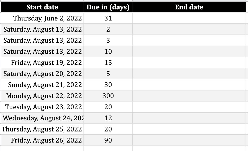
But what if there are many different events that you have to calculate the due date for (like in the screenshot below), then googling one by one can be troublesome.
And that is where Google Sheets can help you out. By applying simple formulas, you can calculate multiple due dates within seconds. In the following, you can read about how to do that.
What are we going to achieve here?
This tutorial will enable you to use Google Sheets to input as many start dates as you want along with the duration in which they’re due.
It will then automatically calculate the due date for you.
Let’s get started
Now, open a blank new Google Sheet and dive into it.
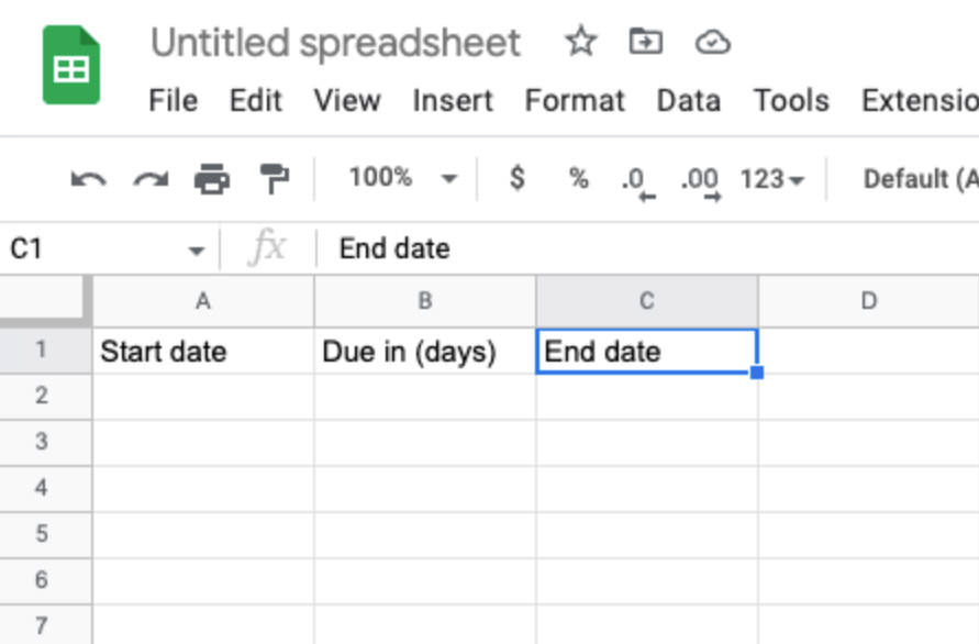
- Insert “Start date“, “Due in (days)“, and “End date” in 3 separate Columns.
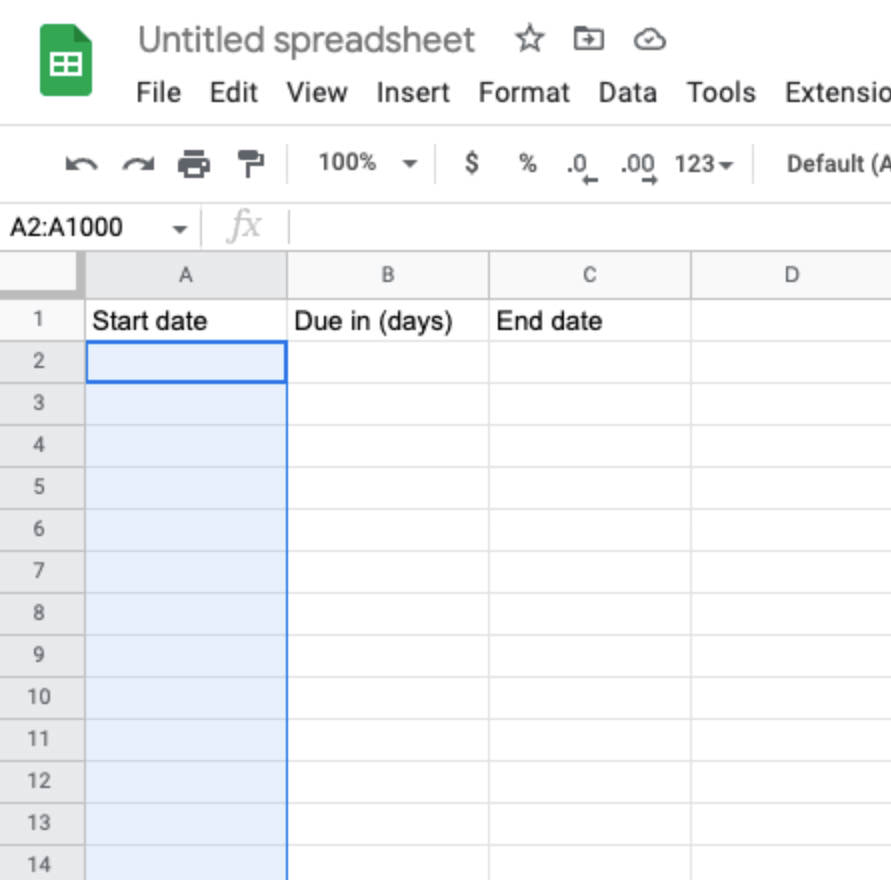
- Click A to select the entire “Start date” Column, hold down Control key (Windows), or Command key (Mac), left click once on “Start date” cell to deselect it.
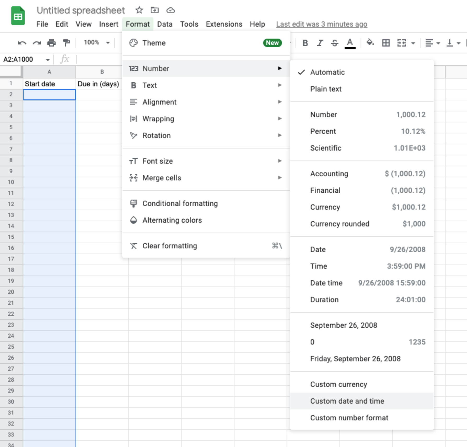
- Go to Format > Number and select Date. This will ensure all cells (except A1) are formatted as
mm/dd/yyyy. If you want to use a different format, go to Format > Number and select Custom date and time. - Repeat step 2 and step 3 for the “End date’ Column.
- Click B to select the entire “Due in” Column, hold down Control key (Windows), or Command key (Mac), left click once on “Due in” cell to deselect it, then go to Format > Number > Number.
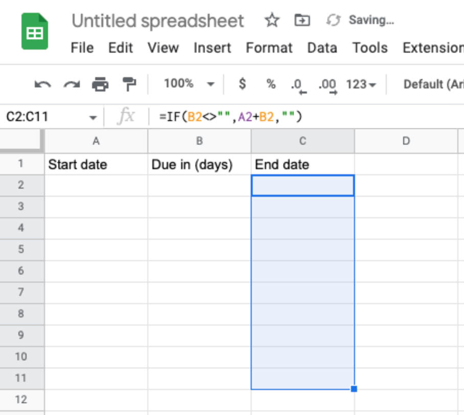
- Now, let’s give it the formula so it calculates the end date for us. Go to the first Column under End date (C2), and enter this formula:
=IF(B2<>"",A2+B2,""), and hit Enter. - Drag this cell down as fast as you want it to go, so the formula applies to other cells as well.
Testing the Sheet
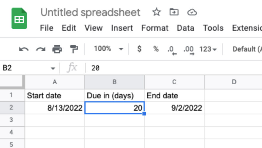
So basically, what the formula does is that when you enter a start date and how long it’s due, Column C displays its end date accurately.
To test the formula we added in Google Sheets with the aforementioned steps, we will enter a start date, say 8/13/2022, and add that it dues in 20 days. The result should show that the end date will be 9/2/2022.
Making it more beautiful
If you’re going to use this feature of Google Sheets more often, then we might as well make it look a little more presentable.
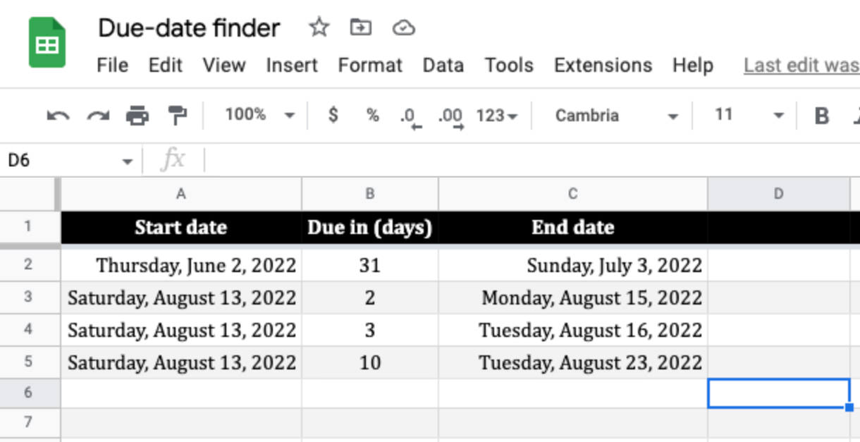
Here are a few things I did to make it neater.
- Replace default font with Cambria, size 11.
- For Row 1, fill color, bold text, and centralized title.
- Freeze Row 1, so it does not move when scrolling. (View > Freeze > 1 row).
- Alternating row colors. (Format > Alternating colors).
Click here to get a copy of the final sample.